44 excel chart change labels
chandoo.org › wp › change-data-labels-in-chartsHow to Change Excel Chart Data Labels to Custom Values? First add data labels to the chart (Layout Ribbon > Data Labels) Define the new data label values in a bunch of cells, like this: Now, click on any data label. This will select "all" data labels. Now click once again. At this point excel will select only one data label. peltiertech.com › multiple-series-in-one-excel-chartMultiple Series in One Excel Chart - Peltier Tech Aug 09, 2016 · XY Scatter charts treat X values as numerical values, and each series can have its own independent X values. Line charts and their ilk treat X values as non-numeric labels, and all series in the chart use the same X labels. Change the range in the Axis Labels dialog, and all series in the chart now use the new X labels.
Change axis labels in a chart - support.microsoft.com Right-click the category labels you want to change, and click Select Data. In the Horizontal (Category) Axis Labels box, click Edit. In the Axis label range box, enter the labels you want to use, separated by commas. For example, type Quarter 1,Quarter 2,Quarter 3,Quarter 4. Change the format of text and numbers in labels

Excel chart change labels
Data Labels in Excel Pivot Chart (Detailed Analysis) Click on the Plus sign right next to the Chart, then from the Data labels, click on the More Options. After that, in the Format Data Labels, click on the Value From Cells. And click on the Select Range. In the next step, select the range of cells B5:B11. Click OK after this. How to Change Axis Labels in Excel (3 Easy Methods) To change the label using this method, follow the steps below: Firstly, right-click the category label and click Select Data. Then, click Edit from the Horizontal (Category) Axis Labels icon. After that, assign the new labels separated with commas and click OK. Now, Your new labels are assigned. EOF
Excel chart change labels. › excel-chart-verticalExcel Chart Vertical Axis Text Labels • My Online Training Hub Apr 14, 2015 · So all we need to do is get that bar chart into our line chart, align the labels to the line chart and then hide the bars. We’ll do this with a dummy series: Copy cells G4:H10 (note row 5 is intentionally blank) > CTRL+C to copy the cells > select the chart > CTRL+V to paste the dummy data into the chart. Edit titles or data labels in a chart - support.microsoft.com The first click selects the data labels for the whole data series, and the second click selects the individual data label. Right-click the data label, and then click Format Data Label or Format Data Labels. Click Label Options if it's not selected, and then select the Reset Label Text check box. Top of Page Excel chart - change data labels reference - Microsoft Q 1/ Select A1:B7 > Inser your Histo. chart 2/ Right-click i.e. on the 1st histo. bar (A) > Add Data Labels (numbers are displayed a the top of the bars) 3/ Click one of the numbers that just displayed (the Format Data Labels pane opens on the right) > Check option "Value From Cells" > Select range C2:C7 > OK > Uncheck option "Value" How to format axis labels as thousands/millions in Excel? 3. Close dialog, now you can see the axis labels are formatted as thousands or millions. Tip: If you just want to format the axis labels as thousands or only millions, you can type #,"K" or #,"M" into Format Code textbox and add it.
Question: labels in an Excel doughnut chart - Microsoft Tech Community Open your Excel document and click on your chart. In the upper bar you will find the "Diagram Tools". Click on the "Design" tab. In the "Data" group, click the "Select data" button. In the right window you will find the "Horizontal axis label". Click on "Edit". Now enter your desired names or values for the legend. › vba › chart-alignment-add-inMove and Align Chart Titles, Labels, Legends ... - Excel Campus Jan 29, 2014 · *Note: Starting in Excel 2013 the chart objects (titles, labels, legends, etc.) are referred to as chart elements, so I will refer to them as elements throughout this article. The Solution The Chart Alignment Add-in is a free tool ( download below ) that allows you to align the chart elements using the arrow keys on the keyboard or alignment ... › clustered-column-chart-in-excelClustered Column Chart in Excel | How to Make ... - EDUCBA E.g., if we change the layout quickly, then just click on the Design tab and click on quick layout and change the layout of the chart. If we want to change the color, we can use a shortcut to change the style and color of the chat; just click on the chart, and there is an option highlighted, as shown below. › documents › excelHow to change chart axis labels' font color and size in Excel? Sometimes, you may want to change labels' font color by positive/negative/0 in an axis in chart. You can get it done with conditional formatting easily as follows: 1. Right click the axis you will change labels by positive/negative/0, and select the Format Axis from right-clicking menu. 2. Do one of below processes based on your Microsoft Excel ...
› how-to-change-axis-values-in-excelHow to Change Axis Values in Excel | Excelchat Change the chart data source. Change the range to both years (2018 and 2019) by clicking on the down-right corner and expanding the selection to the right: Figure 15. Expand the chart data source. Change the values from the x-axis to the “Years” by selecting in the Axis label range cell range I2:J2 (explained in the tutorial above) EOF How to Change Axis Labels in Excel (3 Easy Methods) To change the label using this method, follow the steps below: Firstly, right-click the category label and click Select Data. Then, click Edit from the Horizontal (Category) Axis Labels icon. After that, assign the new labels separated with commas and click OK. Now, Your new labels are assigned. Data Labels in Excel Pivot Chart (Detailed Analysis) Click on the Plus sign right next to the Chart, then from the Data labels, click on the More Options. After that, in the Format Data Labels, click on the Value From Cells. And click on the Select Range. In the next step, select the range of cells B5:B11. Click OK after this.

Excel Course: Inserting Graphs
Charts in Excel - Easy Excel Tutorial
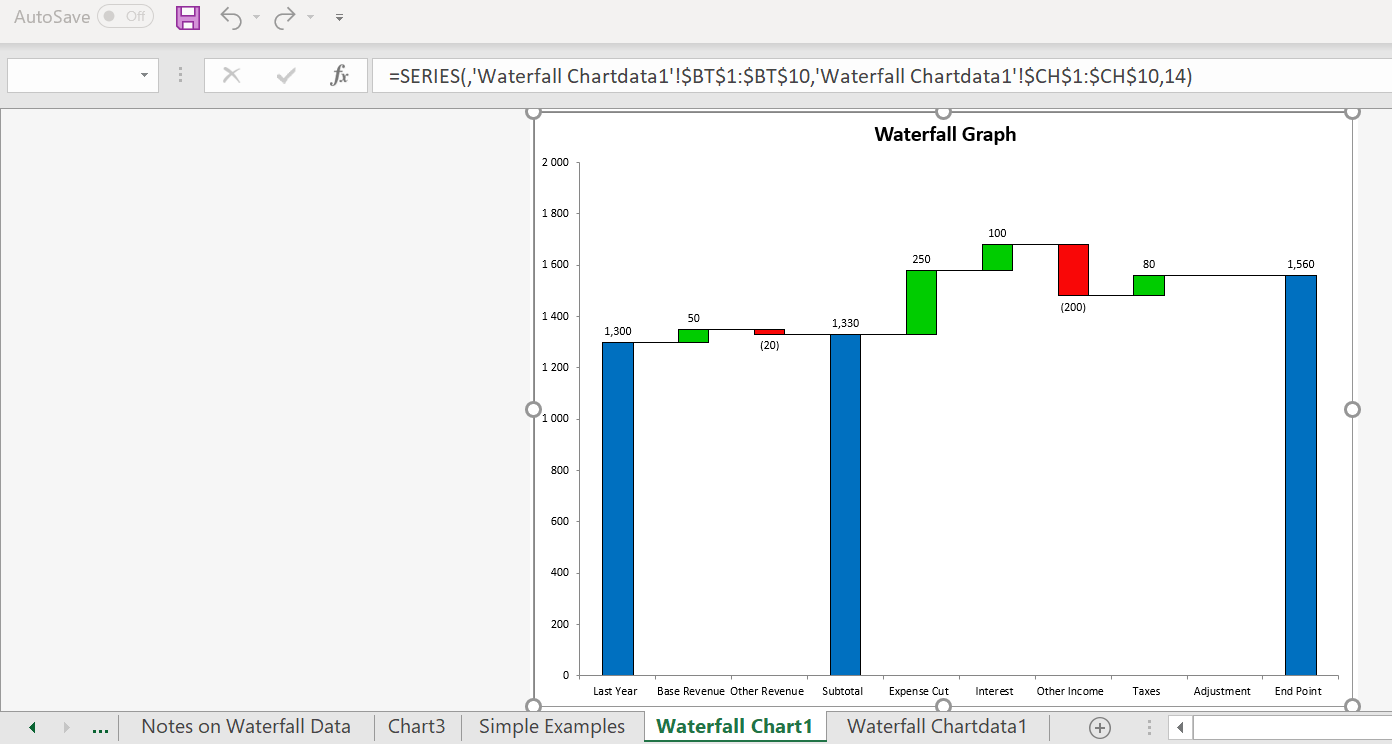
Waterfall Chart Templates (Excel 2010 and 2013) – Edward Bodmer – Project and Corporate Finance
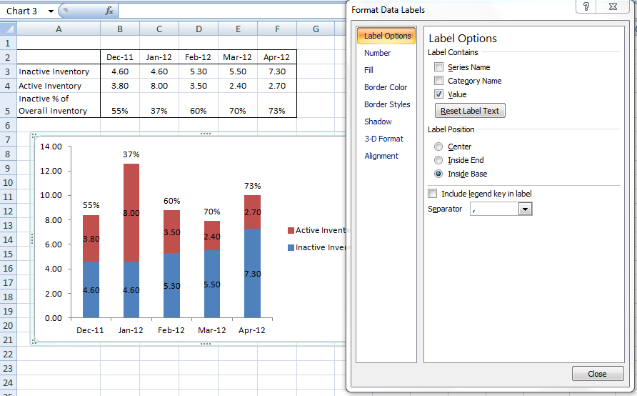
How-to Put Percentage Labels on Top of a Stacked Column Chart - Excel Dashboard Templates

Excel Chart Elements: Parts of Charts in Excel | ExcelDemy
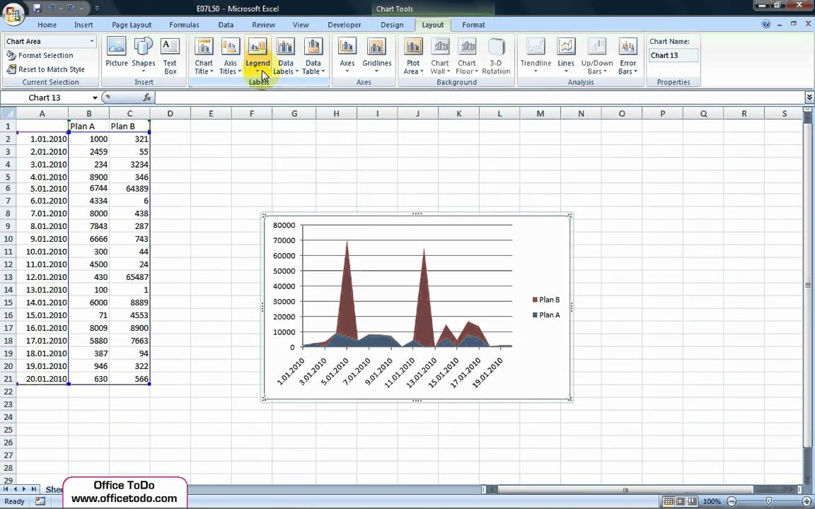
How to add, remove or reposition chart legend? | Excel 2007 - YouTube
Creating a chart with dynamic labels - Microsoft Excel 2016

Excel 2010 Tutorial Changing Chart Labels Microsoft Training Lesson 21.3 - YouTube
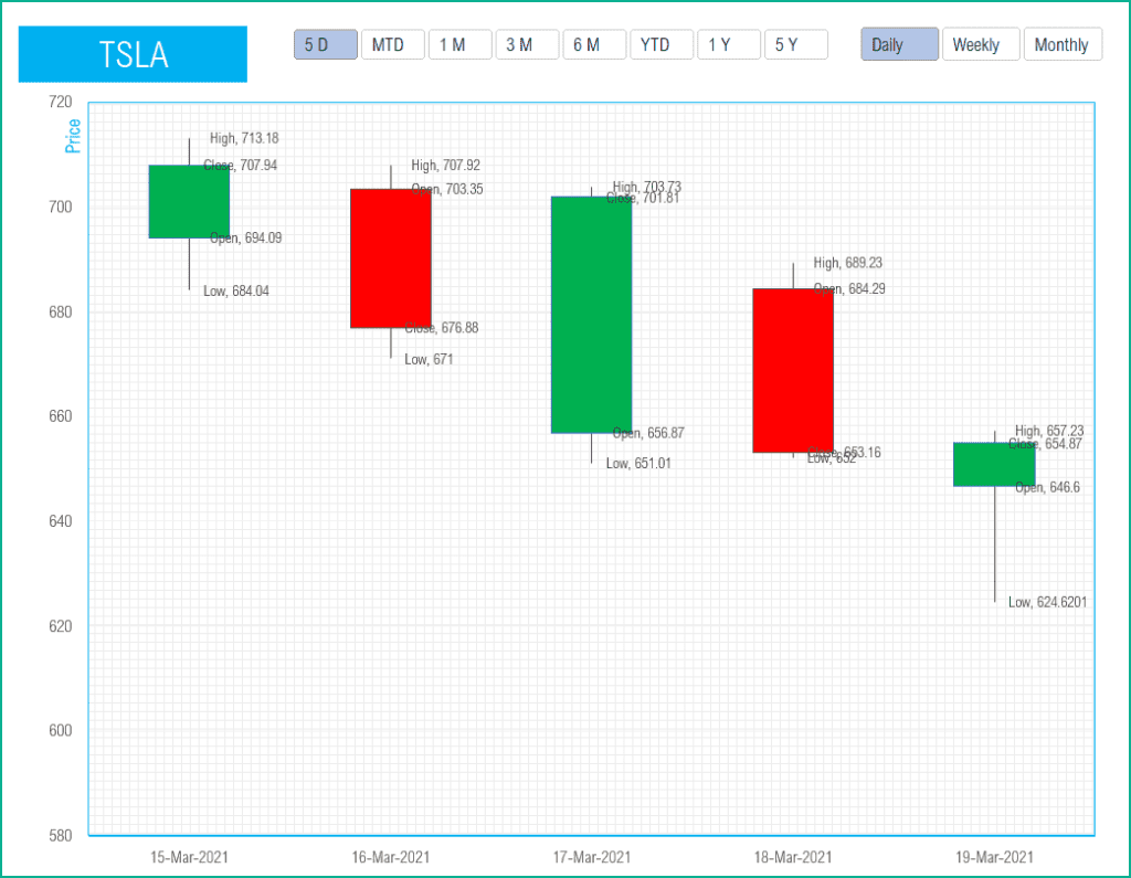
Candlestick Chart Excel Template - Excel for Stock Market

add labels to excel chart 218253.image0 - Top Label Maker
Creating a chart with dynamic labels - Microsoft Excel 2013
How to format the chart axis labels in Excel 2010 - YouTube
Excel Charts: Creating Custom Data Labels - YouTube
Custom Chart Labels Using Excel 2013 | MyExcelOnline

31 What Is A Label In Excel - Labels For Your Ideas
Position Chart Legend & Display Gridlines in Microsoft Excel: MOOC - YouTube
Excel Custom Chart Labels • My Online Training Hub
Post a Comment for "44 excel chart change labels"