40 excel pivot table column labels
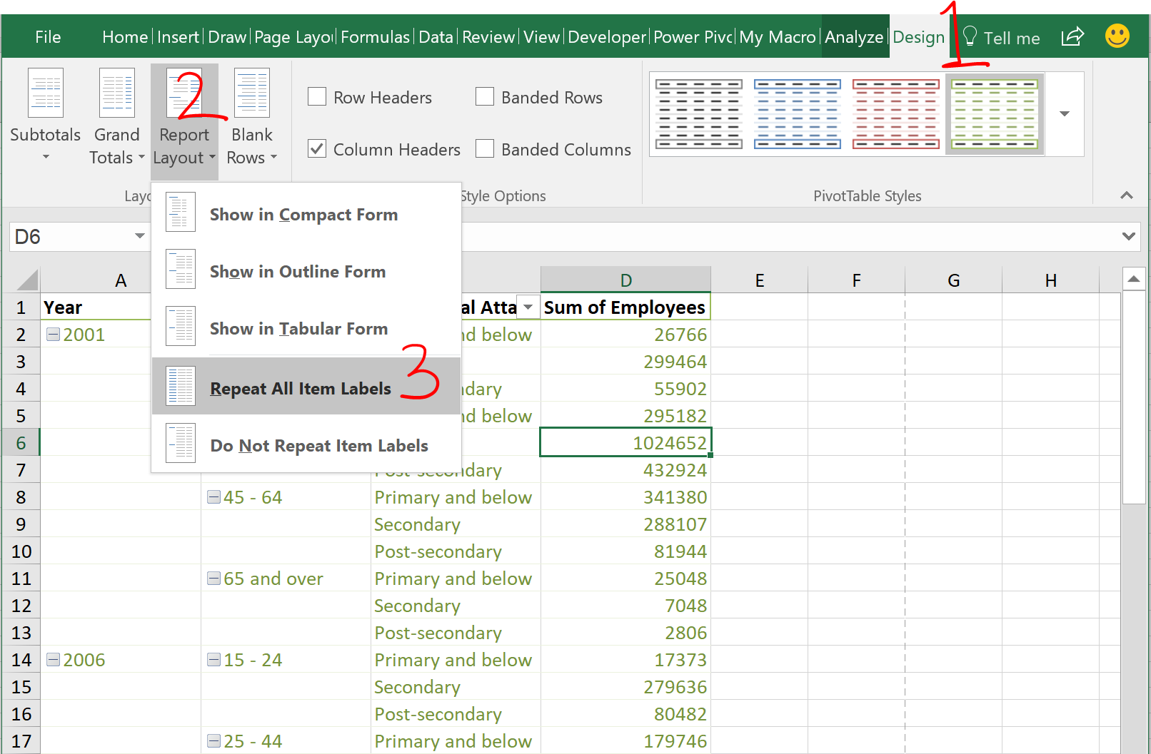
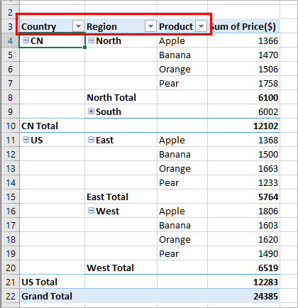
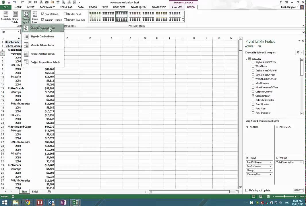
Repeat All Item Labels In An Excel Pivot Table | MyExcelOnline STEP 1: Click in the Pivot Table and choose PivotTable Tools > Options (Excel 2010) or Design (Excel 2013 & 2016) > Report Layouts > Show in Outline/Tabular Form. STEP 2: Now to fill in the empty cells in the Row Labels you need to select PivotTable Tools > Options (Excel 2010) or Design (Excel 2013 & 2016) > Report Layouts > Repeat All Item ... Pivot table row labels in separate columns • AuditExcel.co.za Our preference is rather that the pivot tables are shown in tabular form (all columns separated and next to each other). You can do this by changing the report format. So when you click in the Pivot Table and click on the DESIGN tab one of the options is the Report Layout. Click on this and change it to Tabular form.
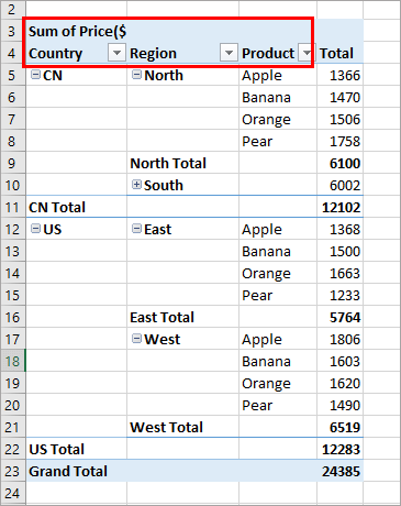
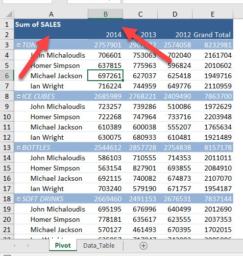
Centre Column Headings in Excel Pivot Table Select a cell in the pivot table On the Ribbon, under the PivotTable Tools tab, click Options At the far left, in the PivotTable group, click Options On the Layout & Format tab, in the Layout section, add a check mark to Merge and Center Cells With Labels Click OK Each Region column label is now centred over its Value field headings.
Excel pivot table column labels
Repeat item labels in a PivotTable - support.microsoft.com Right-click the row or column label you want to repeat, and click Field Settings. Click the Layout & Print tab, and check the Repeat item labels box. Make sure Show item labels in tabular form is selected. Notes: When you edit any of the repeated labels, the changes you make are applied to all other cells with the same label. How to add column labels in pivot table [SOLVED] Re: How to add column labels in pivot table Here are the steps 1. Add a helper column showing Month Text Just as I have done in Column H 2. Now insert a Pivot Table 3. Put Fields in there required sections in the Pivot table Field List Window just as I have done . 4. How to Group Columns in Excel Pivot Table (2 Methods) Steps: First, go to the source dataset and press Ctrl + T. Next the Create Table dialog box will pop up. Check the range of the table is specified correctly, then press OK. As a result, the below table is created. Now, from Excel Ribbon, go to Data > From Table/Range. Then the Power Query Editor window will show up.
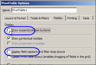
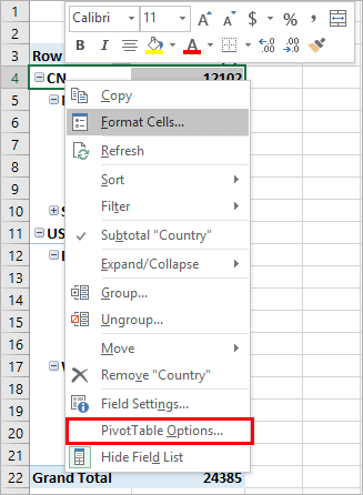
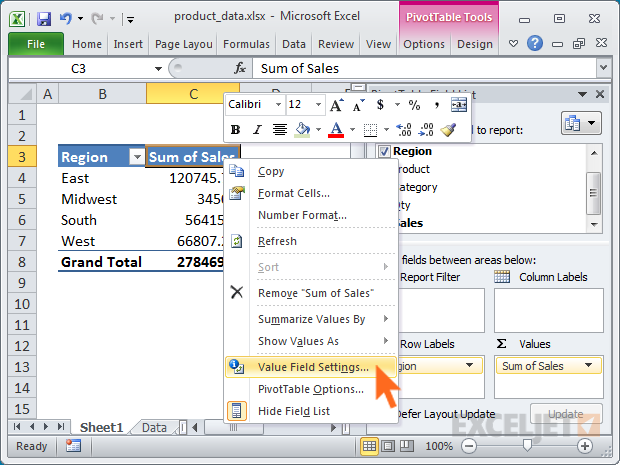
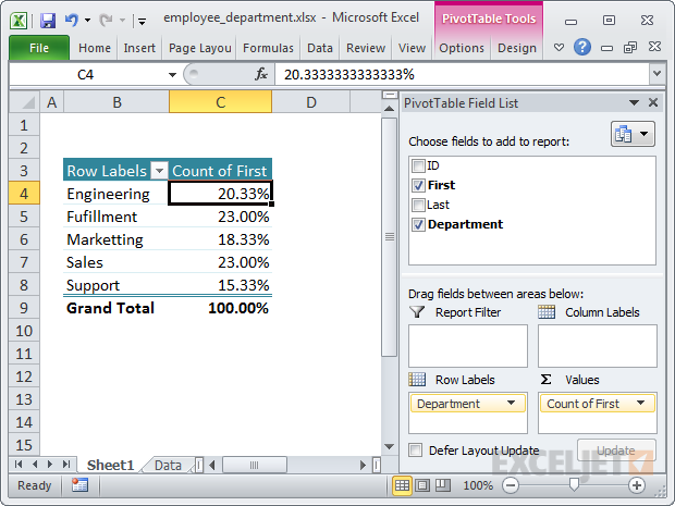
Excel pivot table column labels. Excel 2016 Pivot table Row and Column Labels - Microsoft Community In Excel 2016 I've found when I create a pivot table it unhelpfully shows 'Row Labels' and 'Column Labels' instead of my field names, although in the top left cell it says 'Count of' and then inserts the correct field name. Years ago when I last used Excel it automatically put the field names in all three heading cells. How to repeat row labels for group in pivot table? - ExtendOffice 1. Firstly, you need to expand the row labels as outline form as above steps shows, and click one row label which you want to repeat in your pivot table. 2. Then right click and choose Field Settings from the context menu, see screenshot: 3. In the Field Settings dialog box, click Layout & Print tab, then check Repeat item labels, see ... Hide Pivot Table Buttons and Labels - Contextures Blog Right-click a cell in the pivot table and, in the pop up menu, click PivotTable Options. In the Display section, remove the check mark from Show Expand/Collapse Buttons. This change will hide the Expand/Collapse buttons to the left of the outer Row Labels and Column Labels. Next, remove the check mark from Display Field Captions and Filter Drop ... How to rename group or row labels in Excel PivotTable? - ExtendOffice To rename Row Labels, you need to go to the Active Field textbox. 1. Click at the PivotTable, then click Analyze tab and go to the Active Field textbox. 2. Now in the Active Field textbox, the active field name is displayed, you can change it in the textbox.
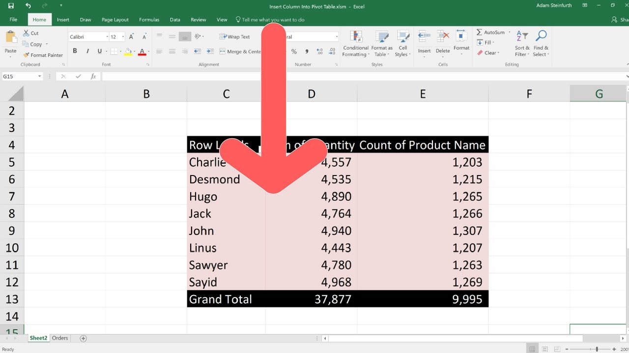
Rename a field or item in a PivotTable or PivotChart PivotChart report Click the object in the chart (such as a bar, line, or column) that corresponds to the field or item that you want to rename. Go to PivotTable Tools > Analyze, and in the Active Field group, click the Active Field text box. If you're using Excel 2007-2010, go to PivotTable Tools > Options. Type a new name. Press ENTER. Automatic Row And Column Pivot Table Labels - How To Excel At Excel Select the data set you want to use for your table The first thing to do is put your cursor somewhere in your data list Select the Insert Tab Hit Pivot Table icon Next select Pivot Table option Select a table or range option Select to put your Table on a New Worksheet or on the current one, for this tutorial select the first option Click Ok How To Filter Column Labels With VBA In An Excel Pivot Table 1. In Excel I have been able to filter the row labels in a pivot table with this code: Dim PT as PivotTable Set PT = ActiveSheet.PivotTables ("Pivot1") With PT .ManualUpdate=True .ClearAllFiters .PivotFields ("App").PivotFilters.Add Type:=xlCaptionDoesNotContain, Value1:=" (Blank)" End With. I need to do the same filter for the column labels ... Use column labels from an Excel table as the rows in a Pivot Table ... Highlight your current table, including the headers Then from the Data section of the ribbon, select From Table Highlight all the columns containing data, but not the Year column, and then select Unpivot Columns Close the dialog and keep the changes. Excel should place the unpivoted data into a new worksheet, looking something like this:
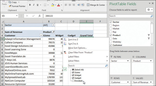
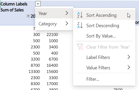
Pivot table row labels side by side - Excel Tutorials - OfficeTuts Excel 3. Now, let's create a pivot table ( Insert >> Tables >> Pivot Table) and check all the values in Pivot Table Fields. Fields should look like this. Right-click inside a pivot table and choose PivotTable Options…. Check data as shown on the image below. The table is going to change. The pivot table is almost ready. Pivot Table column label from horizontal to vertical Pivot Table column label from horizontal to vertical After pivot table and with grouping, some column labels have been showed but the caption is on the top. What i want is put the column header at the left of the row as vertical red text show as below. However, i cannot do this, it said "We cant change this part of pivot table". Sort data in a PivotTable or PivotChart - support.microsoft.com In a PivotTable, click the small arrow next to Row Labels and Column Labels cells. Click a field in the row or column you want to sort. Click the arrow on Row Labels or Column Labels, and then click the sort option you want. ... Excel has day-of-the-week and month-of-the year custom lists, ... How to Move Excel Pivot Table Labels Quick Tricks - Contextures Excel Tips Use Menu Commands to Move Label. To move a pivot table label to a different position in the list, you can use commands in the right-click menu: Right-click on the label that you want to move. Click the Move command. Click one of the Move subcommands, such as Move [item name] Up. The existing labels shift down, and the moved label takes its new ...
Grouping, sorting, and filtering pivot data | Microsoft Press ...
multiple fields as row labels on the same level in pivot table Excel ... multiple fields as row labels on the same level in pivot table Excel 2016. I am using Excel 2016. I have data that lists product models along with relevant data and also production volumes by month. Part of the relevant data are about 5 common part columns with the part # that applies to each model under the appropriate column.
Multi-level Pivot Table in Excel (In Easy Steps)
How to Customize Your Excel Pivot Chart Data Labels - dummies The Data Labels command on the Design tab's Add Chart Element menu in Excel allows you to label data markers with values from your pivot table. When you click the command button, Excel displays a menu with commands corresponding to locations for the data labels: None, Center, Left, Right, Above, and Below.

Repeat all item labels in Pivot Table (aka Fill in the blanks ...
vba sorting pivot table columns by column field label (a date) Hi all, I have a pivot table with multiple row fields and multiple column fields. One of the column fields is a Date and I need some VBA that will auto-sort the columns into ascending order by the Date column field. E.g., if the first four column labels are "2-Jun-2010, 13-May-2009...
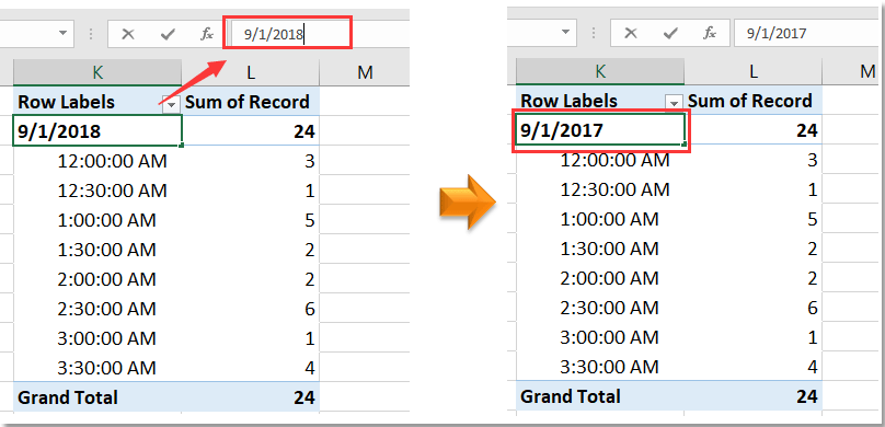
How to rename group or row labels in Excel PivotTable?
How to Use Excel Pivot Table Label Filters - Contextures Excel Tips In an Excel pivot table, you might want to hide one or more of the items in a Row field or Column field. To do that, you could click the drop down arrow for the Row or Column Labels, to see the list of pivot items in that pivot field. Then, in the list, remove the check mark for items you want to remove.
Instructions for Sorting a Pivot Table by Two Columns | Excelchat
Hide Excel Pivot Table Buttons and Labels Right-click any cell in the pivot table In the pop-up menu, click PivotTable Options In the PivotTable Options dialog box, click the Display tab To hide all of the expand/collapse buttons in the pivot table: Remove the check mark from the option, Show expand/collapse buttons
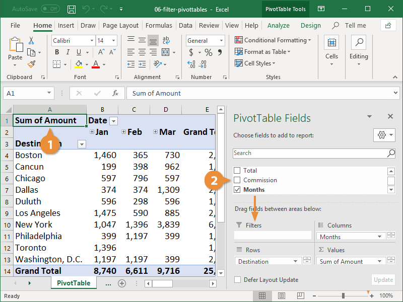
Pivot Table Filter | CustomGuide
Format column labels in pivot table | MrExcel Message Board In an Excel 2007 pivot table, how can I format just the column labels to change the font? I can't seem to select just the labels. Thanks. Forums. New posts Search forums. What's new. New posts New Excel articles Latest activity. New posts. Excel Articles. Latest reviews Search Excel articles.
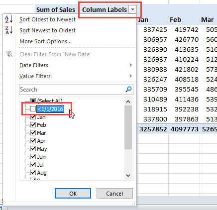
Filter Pivot Table Columns Labels - Excel Dashboard Templates
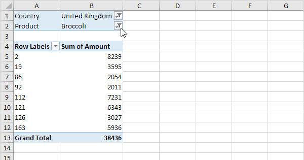
Filter data in a PivotTable - support.microsoft.com In Excel, use slicers and other ways to filter large amounts of PivotTable data to show a smaller portion of that data for in-depth analysis. ... Select any cell within the PivotTable, then go to Pivot Table ... In the PivotTable, click the arrow next to Row Labels or Column Labels. Right-click an item in the selection, and then click Filter ...

Excel Pivot Tables: Insert Calculated Fields & Calculated ...
Data Labels in Excel Pivot Chart (Detailed Analysis) 7 Suitable Examples with Data Labels in Excel Pivot Chart Considering All Factors 1. Adding Data Labels in Pivot Chart 2. Set Cell Values as Data Labels 3. Showing Percentages as Data Labels 4. Changing Appearance of Pivot Chart Labels 5. Changing Background of Data Labels 6. Dynamic Pivot Chart Data Labels with Slicers 7.

Pivot table row labels side by side – Excel Tutorials
Design the layout and format of a PivotTable Change a PivotTable to compact, outline, or tabular form Change the way item labels are displayed in a layout form Change the field arrangement in a PivotTable Add fields to a PivotTable Copy fields in a PivotTable Rearrange fields in a PivotTable Remove fields from a PivotTable Change the layout of columns, rows, and subtotals

How to Sort Data in a Pivot Table | Excelchat
How to make row labels on same line in pivot table? - ExtendOffice Make row labels on same line with PivotTable Options You can also go to the PivotTable Options dialog box to set an option to finish this operation. 1. Click any one cell in the pivot table, and right click to choose PivotTable Options, see screenshot: 2.
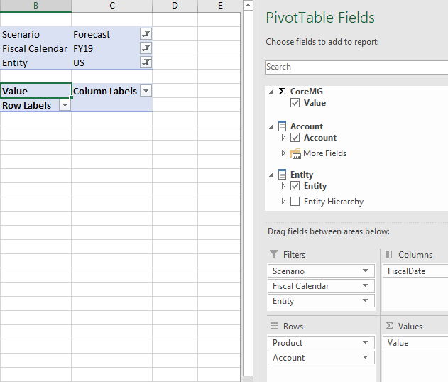
Why is there no Data in my PivotTable? – Kepion Support Center
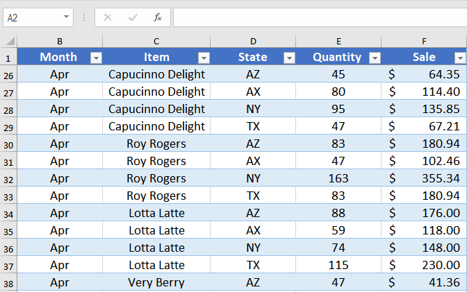
How to Group Columns in Excel Pivot Table (2 Methods) Steps: First, go to the source dataset and press Ctrl + T. Next the Create Table dialog box will pop up. Check the range of the table is specified correctly, then press OK. As a result, the below table is created. Now, from Excel Ribbon, go to Data > From Table/Range. Then the Power Query Editor window will show up.
Repeat all item labels in Pivot Table (aka Fill in the blanks ...
How to add column labels in pivot table [SOLVED] Re: How to add column labels in pivot table Here are the steps 1. Add a helper column showing Month Text Just as I have done in Column H 2. Now insert a Pivot Table 3. Put Fields in there required sections in the Pivot table Field List Window just as I have done . 4.

VBA to grab Pivot Table Column Names | MrExcel Message Board
Repeat item labels in a PivotTable - support.microsoft.com Right-click the row or column label you want to repeat, and click Field Settings. Click the Layout & Print tab, and check the Repeat item labels box. Make sure Show item labels in tabular form is selected. Notes: When you edit any of the repeated labels, the changes you make are applied to all other cells with the same label.
Centre Column Headings in Excel Pivot Table | Excel Pivot Tables
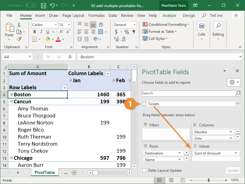
Add Multiple Columns to a Pivot Table | CustomGuide
Hide Pivot Table Buttons and Labels – Contextures Blog
MS Excel 2013: Display the fields in the Values Section in ...
How to make row labels on same line in pivot table?
Design the layout and format of a PivotTable
Excel Pivot Tables - Add a Column with Custom Text
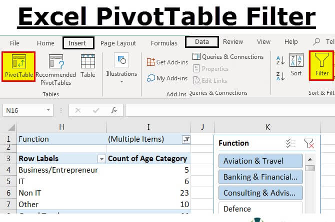
Pivot Table Filter in Excel | How to Filter Data in a Pivot ...

Pivot table row labels in separate columns • AuditExcel.co.za
How to make row labels on same line in pivot table?
Pivot Table Tips | Exceljet

Pivot table row labels in separate columns • AuditExcel.co.za

Microsoft Excel – showing field names as headings rather than ...
How to Flatten and repeat Row Labels in a Pivot Table

Removing old Row and Column Items from the Pivot Table ...

Pivot table row labels in separate columns • AuditExcel.co.za

How to use another column as X axis label when you plot pivot ...
How to make row labels on same line in pivot table?
Pivot Table Tips | Exceljet
Show/Hide Field Headers in Excel Pivot Tables | MyExcelOnline

Pivot Table column label from horizontal to vertical ...

In pivot tables how can I replace Row Labels with field names ...
Microsoft Excel Training in Columbus | Make Tech Easy With EasyIT
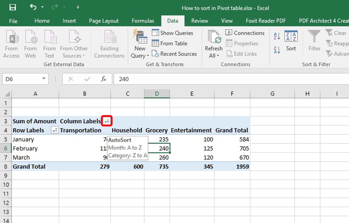
How to Sort Pivot Table | Custom Sort Pivot Table | A-Z, Z-A ...

How to Show Hide Field Header In Pivot Table in Excel

Fix Excel Pivot Table Missing Data Field Settings

Pivot Table headings that say column/ row instead of actual label
Post a Comment for "40 excel pivot table column labels"